


To obtain Return on Investments(RoI) has become increasingly important for any kind of business.
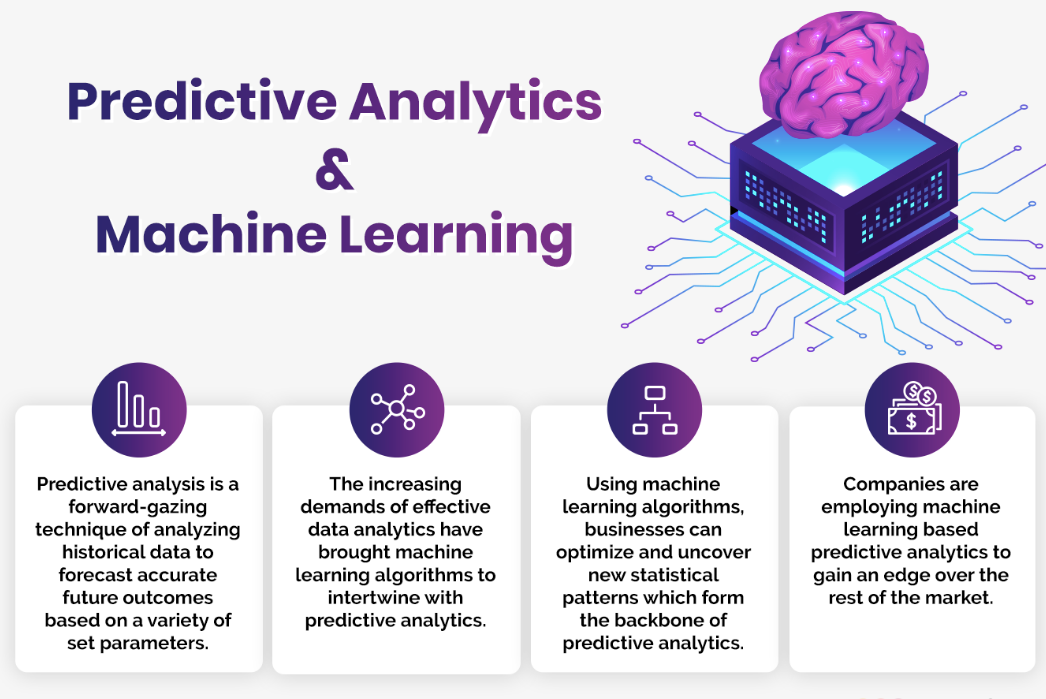
Predictive analytics can become the solution of the hour when it comes to target profitable RoIs. Descriptive Analytics can no longer sustain the various demands of an ever-changing business ecosystem. Your business can no longer rely only on historical data to draw important conclusions relating to your product.
Predictive Analysis on the other hand can take both the historical and the current data to give important insights about the future behaviour. It helps you to calculate the risks and the opportunities which your initiatives hold and intervene them at the right point in time. Thus, ensuring huge ROI.
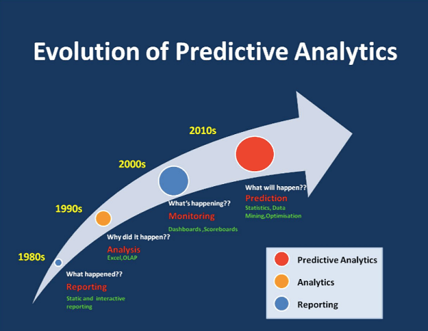
Predictive Analytics has been here for a while but its use cases are still getting explored. A large number of use cases have already been explored by Queppelin in the fields of marketing, finance, manufacturing and energy consumption. After building applications based on Predictive Analytics Queppelin helped its clientele to increase their revenues and cut down their loss.
Thus, even after delivering the model to our clients, the model keeps learning from the new data that comes in.
Queppelin uses Exploratory Data Analysis(EDA) to conduct initial stage research on data to discover trends and patterns, to find similarities, repeated outcomes or responses for future predictions. EDA helps us to evaluate data collections, mostly using visual tools, to outline their key characteristics.
Before using data for analysis, the aim of analysing the same should be clear. Our analysis is very much client-centric. We evaluate various relations between variables that are especially important or unpredictable. EDA also takes care of problems with the gathered data, such as measurement error or missing data, etc. Subsequently, we analyse the data and visualize it by plotting charts, graphs and diagrams wherever necessary. Plotting data in the form of such visual representations makes it easier for both the client and Queppelin to understand the underlying patterns in the data.
One of the most recurring forms of data is Time Series Data. Time series is a series of data points in relation with time in which time is often the independent variable. Stationarity is a crucial aspect of time series. If the statistical properties of a time series do not change over time, then the data series is said to be stationary. In other terms, a stationary time series has constant mean and variance. Thus, the statistical stationarity test is done for the data plots. For determining the stationary or non-stationary nature of a time series, a statistical test known as Dicky-Fuller test is carried out on the data plot.
The test checks the null hypothesis of an autoregressive model getting a unit root. If a root is present, then p >0, and the process is not stationary. Otherwise, p=0, the null hypothesis is rejected and the process is said to be stationary. Ideally, it is beneficial to have a stationary time series for modelling. But since not all of them are stationary, different changes can be done to make these models stationary.
From the plots made using data gathered, several time series patterns can be observed. Trend and seasonality are two of these.
Trend is the existence of long term increase or decrease in the data. It generally follows the same kind of path with changing time.
Seasonality refers to the existence of a seasonal pattern with similar intervals of time like daily, weekly, monthly, quarterly, etc. Seasonality always has a fixed and known frequency. Seasonality is observed when time series data shows unvarying and certain patterns at specific time intervals. An example of seasonality in time series is retail sales, which generally rise between September to December and fall between January and February. This pattern is seen almost every year through recorded data, showing the time series to be seasonal in nature.
All time series are not stationary and such data plots are made to undergo changes by applying methods to make them stationary. For this purpose, the time series being studied is modelled in order to make predictions using methods like
Some of them are explained below:
Autocorrelation shows the relation between a time series and its past values. On the other hand, Autocorrelation function plot refers to how a time series is related with itself i.e. a plot also including the ls unit. The ACF plot is used to determine whether to use the AR term or MA term in the ARIMA model. The two are used together very rarely.
If there is a positive autocorrelation at lag 1, then the AR model is used. If there is a negative autocorrelation at lag 1, then the MA model is used. Using the Autoregressive (AR) component: A complete AR model does forecasting only while using past values similar to linear regression where AR terms used are directly proportional to the periods considered.
Using the Moving Averages (MA) component:
A complete MA model smoothens the effect of sudden jumps in values of data seen in a time series plot. These jumps represent the errors calculated in the ARIMA model.
Integrated component:
When the time series is non-stationary, this component is considered. The parameter for the integrated component is the number of times difference has to be taken to make the time series stationary.
Seasonal ARIMA models (Also known as SARIMA) : This model is brought into use when the time series shows seasonality. Like the ARIMA model, SARIMA model too has certain parameters. These are p,d,q, which refer to the same terms as described above in the ARIMA model. m denotes the number of periods in every season.
P,D,Q refer to p,d,q for the seasonal part of the time series.
Seasonal differencing considers the seasons and finds out the differences in the current value and the value of the same in the preceding season. For eg. differencing in the monthly sale of a certain item in December will be value in December 2019 – value in December 2018.
Data pipeline in simple words is a system comprising different parts to carry out a combined process of enabling movement of raw data into the system from one end and giving processed, useful data for predictions and analysis from the other end.
We can assume a data pipeline analogous to a filtration water pipeline in which water enters from one end, many purification and filtration processes take place on the water and purified water is given as output from the other opening.
The model that has been worked upon needs timely updating and modification for better results with every change. Data pipelines are enhancing the productivity, marketing, sales, personalized consumer interaction and services of many companies across the world because of this innovative approach of data science
Long Short Term Memory Networks(LSTM) invoke the context-aware behavior in Artificial Neural Networks(ANNs). LSTMs store what they learn and propagate it through computer memory and a special type of network architecture facilitates the propagation of learned parameters forward. What is quite unique about human memory, also makes LSTMs special which allows them to forget whatever isn’t important through their forget gate. This is how they overcome the problem of remembering very large contexts.
The image depicts a typical LSTM cell. Xt denotes the present input at time t, Ht is the input from the previous cell (for overtime memoization). The LSTM calculates the degree to which the previous information should be forgotten and the extent to which the current information is to be updated with the previous information using sigmoid activation ( to keep the extent of forgetting and updation between 0 and 1). A deeper dive into LSTMs can be found here for proper understanding.
Simple LSTMs find extensive use cases in Predictive analysis but cannot deal with a lot of use cases. Thus, at Queppelin we experimented with Bayesian Forecasting. Bayesian Forecasting is another method for time series forecasting. This approach allows us to use prior probabilities and reduces the problem of overfitting which is commonly faced in Artificial Neural Networks with a large number of parameters. Further, the problem of overfitting is a major setback, that makes relying on ANNs an issue. One solution to the overfitting problem is to take a Bayesian approach which allows us to impose certain priors on our variables.
A machine learning system helps to carry out an end-to-end flow of the data. Pipelines manage the automation and flow of data along with the Machine Learning Models. Pipelines are modular data flow management tools that help us build and manage production-grade autonomous Machine Learning Algorithms.
In Machine Learning Pipelines, each of the steps is iterative and cyclical. The main objective of a machine learning pipeline is to build a high-performance scalable, fault-tolerant algorithm. The entire process should be developed optimizing latency and modes of data ingress ( online[real time] or offline[batch-processing] ).
The first step that we follow is we define the business problem and its requirements. That is to say, the mode of data ingress, the type of dataset, the preparatory steps involved, and the evaluation metrics to analyze performance.
Data Ingestion
The local endpoints and the source of data is to be programmed to the algorithm, along with the type of ingestion – Online or Offline.
Data Preparation
This is the step where we process the data and extract features along with the selection of attributes.
Data Segregation
This is the stage where we layout the map for splitting the data for training, testing and validation purpose on new data as compared to previous cycles of the algorithm, in order to analyze and optimize performance through hyperparameters
Model Training
In this step, because of the modular nature of the pipeline, we are able to plug and fit multiple models and test them out on the training data.
Candidate Model Evaluation
Here we aim at assessing the performance of the model using test and validation subsets of data. It is an iterative process and various algorithms are to be tested until we get a Model that sufficiently fulfills the demand.
Model Deployment
After the model is chosen based on the most accurate performance, it is generally exposed through APIs and is then integrated alongside decision-making frameworks as a part of an end-to-end analytics solution.
Performance Monitoring
This is the most important stage as here, the model is continuously monitored to observe how it behaves in the real world. Then the calibration and new data collection take place to incrementally improve the model and its accuracy on generalization.
Model Training:
Predictive Analysis utilises the technique of predictive modeling to use computational and mathematical methods to come up with Predictive models. The predictive models examine both the current and the historical data to understand the underlying pattern in the two datasets. Thus, making forecasts, predictions or classification of future events in real time.The model updates with the arrival of new data.
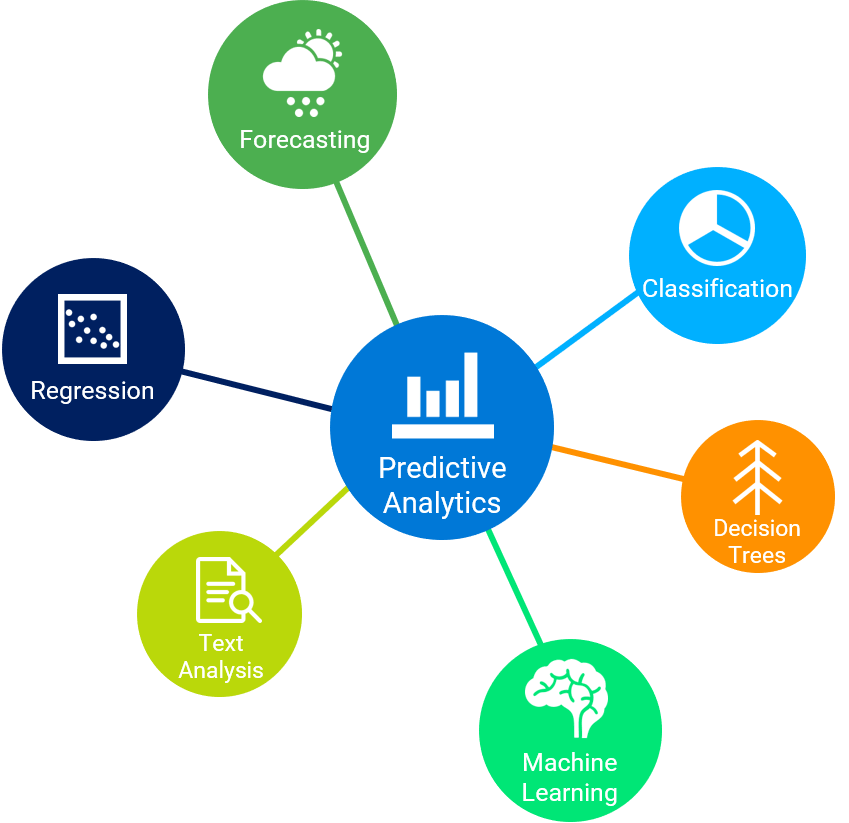
Predictive modeling is the heart of Predictive Analysis. Queppelin makes every effort to create the right predictive model with the right data and variables. Some common types of models:
A predictive model runs one or more Machine Learning and Deep Learning algorithms on the given data through an iterative process. Some of those are:
The models and algorithms described above learn parameters suiting the data that they receive. We need to choose some of them which do not come directly from the data. Such parameters are called hyperparameters and their values are set before training begins. Queppelin utilises its expertise to come up with the best hyperparameters so that your model outperforms the state-of-the art models.
Hyperparameter tuning involves optimizing the hyperparameters by conducting a search in the hyperparameter space, i.e, training the model and then evaluating the model for each set of these parameters.
Model fine tuning with various data-lag values to have the best accuracy Subjective to performance
After we are done building and training your model and setting the hyperparameters, we need to evaluate the same. This process is called backtesting. The later part of the test data is segregated and kept to help us evaluate the model. It thus leverages time series data and non-randomized splits in the data.
Developing Accuracy metrics for data points Test on different time series samples from the past Overall Performance Measurement Metrics
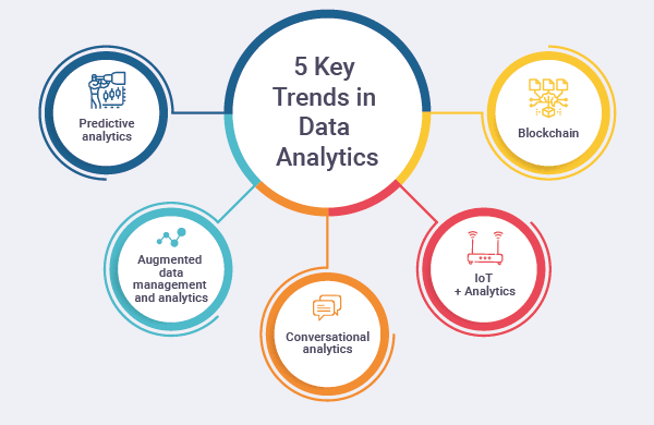
We are constantly exploring the possible and unprecedented use cases that Predictive Analysis can have in various businesses. Some of those are:
Solar energy is becoming an increasingly reliable source of energy and is gaining enough traction already. Businesses owning large-scale Solar Plant farms can suffer huge losses due to the volatility of the Photovoltaic cells during bad weather conditions. Thus, accurate forecasting of the energy production is necessary to manage power grid production, delivery and storage.
The increasing amount of water flowing into the Arctic Ocean can cause significant thermohaline circulation collapse and unpredictable climatic conditions. The ocean ecosystem has a vital role to play in the climate but very little is known about the predictability of climate change. Thus, using forecasting models we can predict the inflow of freshwater into the ocean.
The use cases of Predictive Analysis is very important in the finance industry. The forex rates change at a very fast pace and if we are able to predict the rates using our Predictive Models, we can scale the profits of a company multifold.